Sign In
News
Click here for updated DEM quality analysis (includes helpful interactive tools)
Many research studies analyzed SRTM quality and published a wide range of RMSE values: 9.73m world-wide, 8.28m in Philippines, 3.53m at 13,305 reference points in US, 3.82m near Hispaniola shoreline, 15.27m at six US sites, and 10.3m at 335 IGS stations.
And, our study around Toronto Pearson Airport published an RMSE of 5.06m. We also analyzed NASADEM, the next generation of SRTM, which presented the airport's main runway as hilly, jagged terrain!
The variance of published RMSE results raise a few questions:
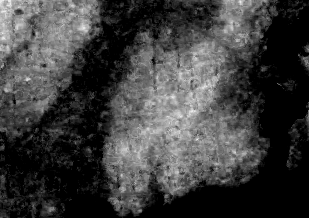
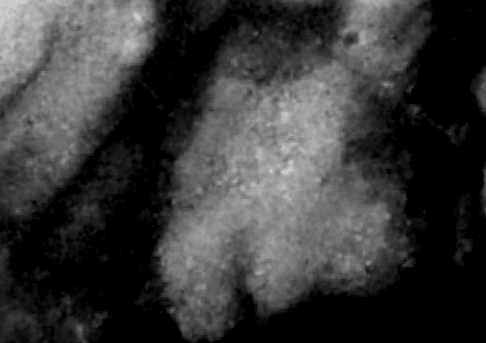
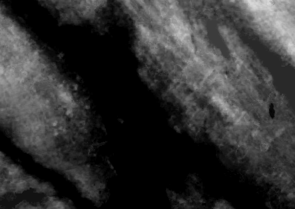
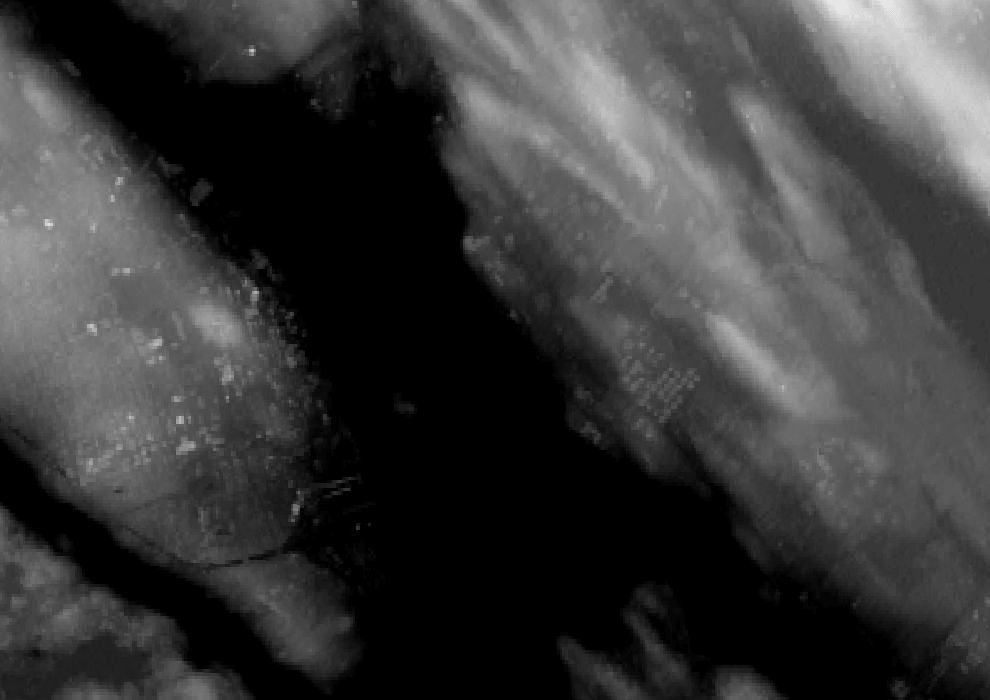
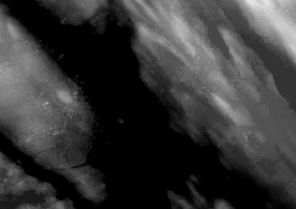
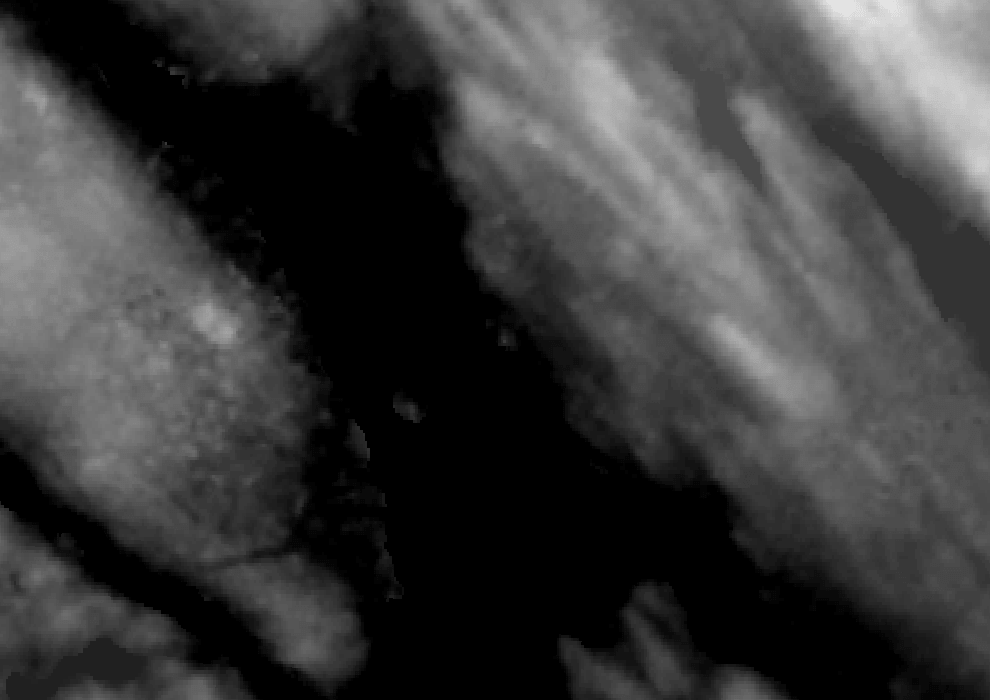
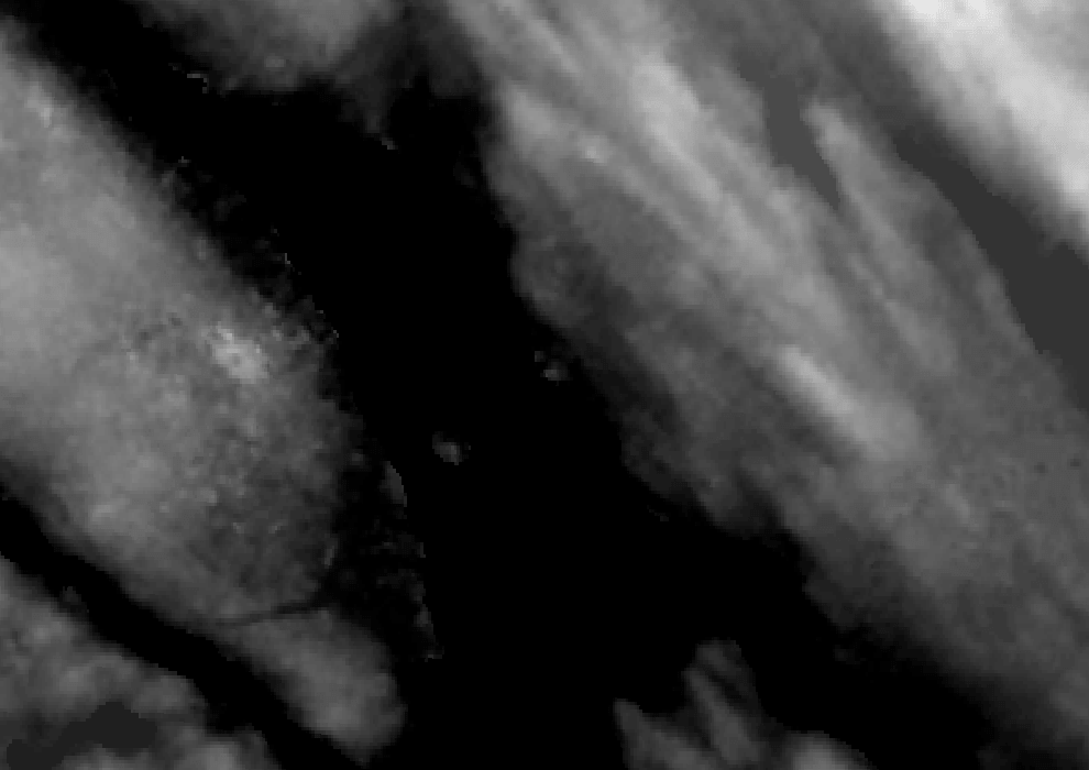
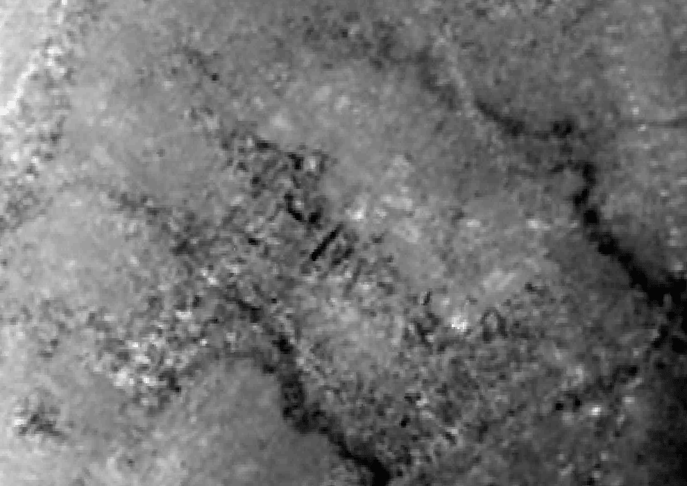
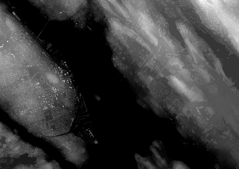
The three scenes below visualize the Digital Elevation Models (DEMs) we studied last week. Each represents 57 km² (9.0 x 6.3 km) of area. Dark areas are low surface elevations; bright areas are high surface elevations. Tiny, bright rectangles are the tops of tall structures, usually buildings. Each scene includes a LIDAR image which depicts the perfect surface DEM. Use the toggle in the top-left corner of each scene to switch between DEMs and discover where each is less than perfect, due to remote sensing errors or surface changes over time.
These 3-D scenes (the 3rd dimension is surface elevation represented as brightness) gives us another perspective into DEM quality. All DEMs have identical 30 m grid spacings but present stark differences in spatial resolution, with some preserving building footprints and others appearing foggy.
Dark areas at the bottom and right are Lake Ontario at 72 m elevation (EGM96). Specular highlights in AW3D30 are building rooftops confirmed by LIDAR, but absent from Copernicus DEM 30.

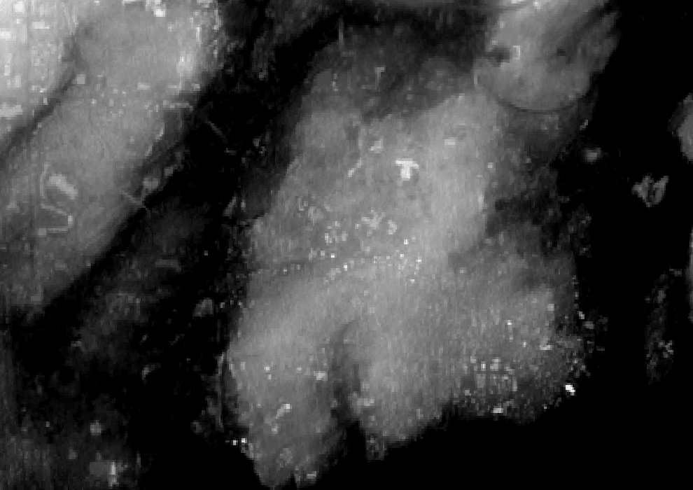
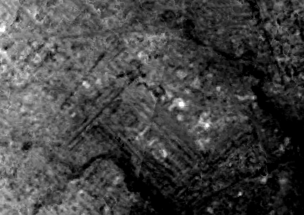
The wide, dark diagonal down the middle is an ocean harbor. LIDAR shows many building rooftops in downtown (left of harbor) and two dozen oil tanks (right of harbor). AW3D30 preserves some of this detail; Copernicus preserves none. This could be because AW3D30 downsampled from a 5 m DEM while Copernicus downsampled from a 12 m DEM.
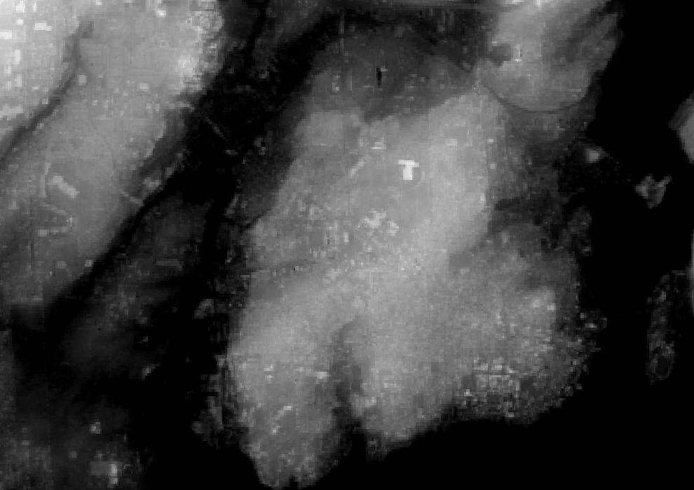
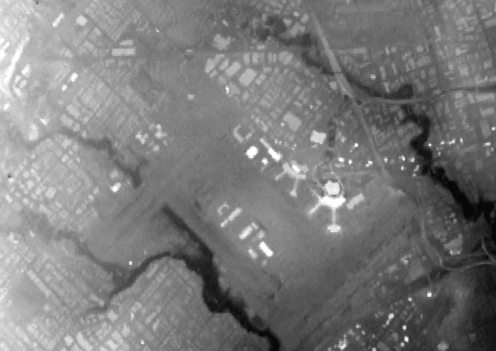
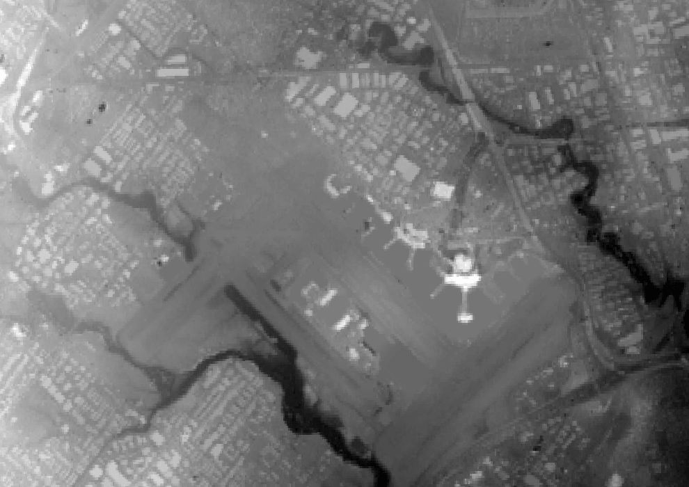
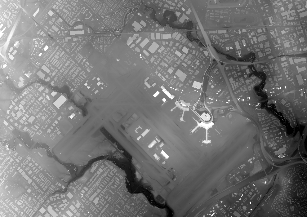
The airport's runways have mild slopes, which should appear free of noise. ASTER has an artifact down the middle, almost vertical; perhaps it's where two strips were merged. As before, AW3D30 preserves building rooftops better than Copernicus, but Copernicus shows much less noise around the runways. SRTM / NASADEM has severe noise, far beyond what we've seen in other areas; both are unusable.
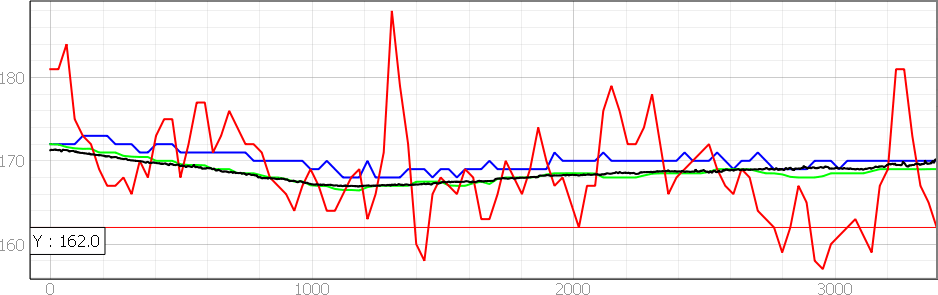
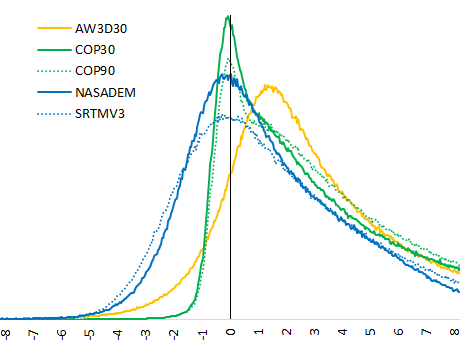
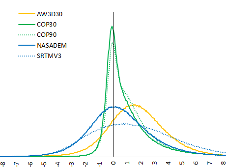
This profile compares DEM elevations to LIDAR (in black) along runway 05/23:
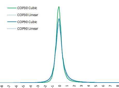
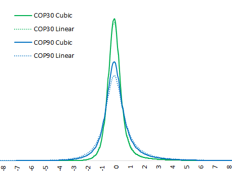
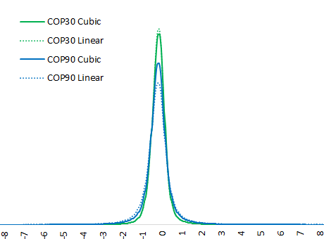
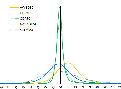
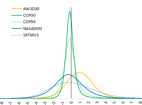
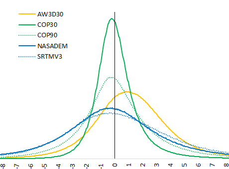
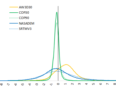
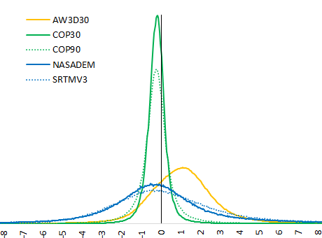
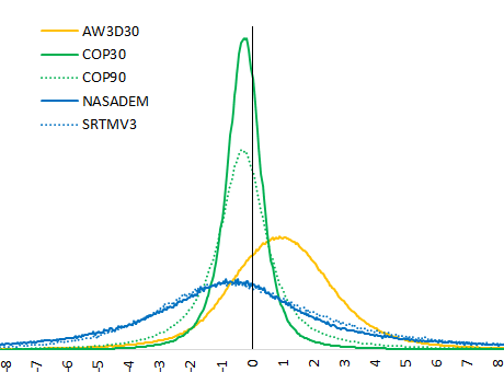
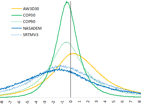
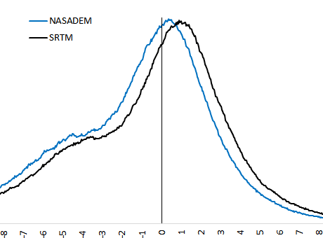
The graphs below plot [ DEM elevation - LIDAR elevation, in meters ] in the 81% of the 57 km² area classified as Urban / built-up by NALCMS 2015 v2. (Our other study compares DEM elevation to ICESat-2 ATL08 terrain elevation.) The right graph pulls SRTM / NASADEM from the left graph to highlight how NASADEM varies from SRTM.
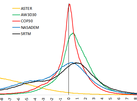
| DEM | Comparisons | RMSE | Mean | StDev | < 2 m | > 8 m |
|---|---|---|---|---|---|---|
| ASTER | 7,358,741 | 12.26 | -10.67 | 6.03 | 4.2% | 68.3% |
| AW3D30 | 7,358,741 | 2.93 | 0.84 | 2.80 | 64.1% | 1.7% |
| COP30 | 7,358,741 | 3.21 | -0.15 | 3.21 | 72.1% | 1.9% |
| NASADEM | 7,358,741 | 5.03 | -1.47 | 4.81 | 44.2% | 8.5% |
| SRTM | 7,358,741 | 5.06 | -0.80 | 4.99 | 41.7% | 8.3% |
The area around Toronto Pearson Airport is relatively flat and vegetation-free, and should present few challenges to remote sensing equipment. Let us know if you have any ideas about what happened with SRTM / NASADEM.
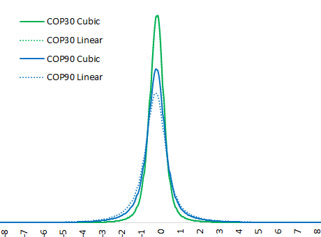
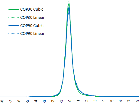
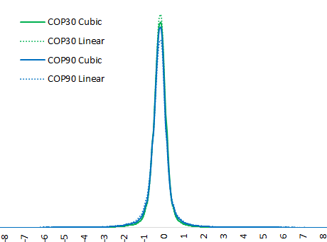
Bicubic fits the earth's curved surfaces better than bilinear interpolation with DEM grids of 30 m or greater. To demonstrate this, we revisit our previous study, this time with bilinear interpolation. This study looks at short vegetation and barren surfaces, which reveal the earth's surface to remote sensing equipment better than other surface types. The results are below:
| Label | DEM | Grid Spacing | Interpolation |
|---|---|---|---|
| CUBIC30 | COPernicus DEM | 30 m | Bicubic |
| LINEAR30 | COPernicus DEM | 30 m | Bilinear |
| CUBIC90 | COPernicus DEM | 90 m | Bicubic |
| LINEAR90 | COPernicus DEM | 90 m | Bilinear |
| Label | Comparisons | RMSE | Mean | StDev | < 2 m | > 8 m |
|---|---|---|---|---|---|---|
| CUBIC30 | 45,115,640 | 1.20 | 0.12 | 1.20 | 97.0% | 0.4% |
| LINEAR30 | 45,122,056 | 1.60 | 0.14 | 1.60 | 97.0% | 0.4% |
| CUBIC90 | 45,115,640 | 1.26 | 0.15 | 1.25 | 95.8% | 0.3% |
| LINEAR90 | 45,121,452 | 1.97 | 0.19 | 1.96 | 95.1% | 0.4% |
| Label | Comparisons | RMSE | Mean | StDev | < 2 m | > 8 m |
|---|---|---|---|---|---|---|
| CUBIC30 | 6,111,149 | 1.22 | -0.12 | 1.21 | 98.5% | 0.3% |
| LINEAR30 | 6,113,683 | 2.37 | -0.07 | 2.37 | 98.4% | 0.3% |
| CUBIC90 | 6,111,149 | 1.30 | -0.12 | 1.29 | 97.6% | 0.3% |
| LINEAR90 | 6,113,648 | 2.64 | -0.08 | 2.63 | 96.9% | 0.4% |
Bilinear has only one advantage over bicubic: speed of computation. Our benchmarks found bilinear to be as fast to four times faster than bicubic interpolation, depending on the percentage of CPU cache misses incurred.
But you might not see these benefits. DEM tiles are very large rasters each covering 1 x 1 degree, with the most north-west elevation at the lowest memory address. If these tiles are accessed randomly, the CPU will spend more time waiting for memory than performing computations. If query throughput is your priority, before replacing bicubic with bilinear interpolation, look at how your program accesses DEM tiles. It should query all locations within one tile before querying the next tile. And within a tile, it should query north-west locations first, then move east and finally south.
Copernicus DEM 30 and 90 are accurate global DEMs. Bilinear interpolation will degrade their accuracy, especially Copernicus DEM 90. If query throughput is a priority, try to reduce CPU cache misses before replacing bicubic with bilinear interpolation.
Digital Elevation Models (DEM) have many uses, from land and forest management, wireless propagation studies and satellite image orthorectification. Flight simulators use one-meter DEMs to deliver state-of-the-art visuals — for only $59.99!
Fortunately we have many DEMs to choose from, including these six which are the subjects of our comparison:
Each DEM has its own strengths, and choosing the the right one depends on evaluating metrics such as
| Metric | Details |
|---|---|
| Vertical accuracy (absolute) | DEM elevation compared to geodetic vertical control points, located across a range of terrain slopes and landcover types. A DEM might perform well in flat, uncluttered spaces but not on forested hillsides |
| Vertical accuracy (relative) | Elevation difference between adjacent DEM cells. Used to derive slope (rise over run) and aspect (slope azimuth) |
| Horizontal uncertainty | Increases error of slope, aspect and other attributes |
| Horizontal skew | A shift in some or all of grid. Can prevent co-registration with landcover or other spatial databases |
| Grid spacing | A 90 m DEM captures fewer terrain details than a 30 m DEM and can compromise terrain modelling, eg. decrease slope gradient |
| Storage / bandwidth | A 90 m DEM uses 1/9th the storage or bandwidth of a 30 m DEM |
| Terrain and / or Surface | Use a Digital Terrain Model (DTM) to analyze water flow and a Digital Surface Model (DSM) to analyze wireless signal propagation. Combine both to measure tree canopy height or forest volume |
| Coverage area | Global or local? 1, 2 or 5 m DEMs might be available only for regional areas of interest |
| Age | Some DEMs (not listed above) are 30+ years old |
| Voids | Peaks can obscure mountain side creating data voids. How many? How were they handled? |
| Security | Was DEM corrupted during download, or otherwise tampered with? Are checksums available? |
| Accessibility | How easy is it to download DEM? Ftp, batch wget or cumbersome website? |
| License | What use cases are allowed or prohibited? Can you make derivative works? |
| Cost | Price can vary from free to thousands of dollars for a regional area of interest |
| Metadata | Is ancillary data provided, eg. waterbody mask? |
| Waterbody | Are lakes flattened to one elevation, river elevations adjusted by a constant interval and shorelines elevated above adjacent waterbody? |
| Updates | All DEMs have errors. How do you report them? How often are updates published? |
| Format | A binary file with 1 arcsecond grid spacing (eg. SRTM) is easy to use via your own bespoke software, but a TIF with a more efficient projection might be easier to use with packaged software |
| Coordinates / datum | Does DEM use an obscure, local projection or vertical datum? |
Our study addresses the first metric above, Vertical accuracy (absolute). We loosely followed the approach of this study which used ICESat-2 ATL08 segments as vertical control points, but with a few changes:
Our study compares 280 million ATL08 segments captured from 2018-Oct-14 to 2020-Sep-30 across North America to the six DEMs above. NALCMS 2015 v2 provided landcover type:
| # Comparisons | Percentage | NALCMS Landcover Type |
|---|---|---|
| 174,238,427 | 62.2% | Short Vegetation |
| 48,308,780 | 17.3% | Needleleaf Forest |
| 28,604,991 | 10.2% | Barren |
| 12,895,184 | 4.6% | Broadleaf Forest |
| 9,683,631 | 3.5% | Mixed Forest |
| 6,208,490 | 2.2% | Urban |
| 279,939,503 | 100.0% | ALL |
| # Comparisons | Percentage | ATL08 terrain_slope |
|---|---|---|
| 87,319,337 | 31.2% | Mild (0.005 - 0.02) |
| 71,503,957 | 25.6% | Flat (< 0.005) |
| 61,059,044 | 21.8% | Moderate (0.02 - 0.05) |
| 39,805,808 | 14.2% | Rugged (0.05 - 0.125) |
| 20,251,357 | 7.2% | Very Rugged (> 0.125) |
| 279,939,503 | 100.0% | ALL |
An ICESat-2 ATL08 segment reports one latitude, one longitude, one terrain and one canopy elevation from where 100s of photons struck a track 14 m wide and 100 m long, at ground level, up in a pervious vegetative canopy — or infrequently way up in the clouds! This process is at the forefront of remote sensing technology and offers an unbelievable volume of data with an unbelievable level of precision. But, what about errors and their distribution? Are they random or have systemic properties? If the 100 m track is flat terrain, we have confidence in the values reported. For rough terrain, our confidence drops. For this reason, we caution you when interpreting any results below where terrain_slope > 0.02 (ie. > 2 m / 100 m).
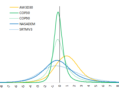
RMSE, Mean, StDev and x-axis are based on [ DEM elevation - ICESat-2 terrain elevation, in meters ]. Graphs omit ASTER as its curves ride near the x-axis (it's not that ASTER is bad; it's that Copernicus DEM is very good!) Toggle the Terrain Slope buttons to see results at various slopes (for uncluttered landcover types only).
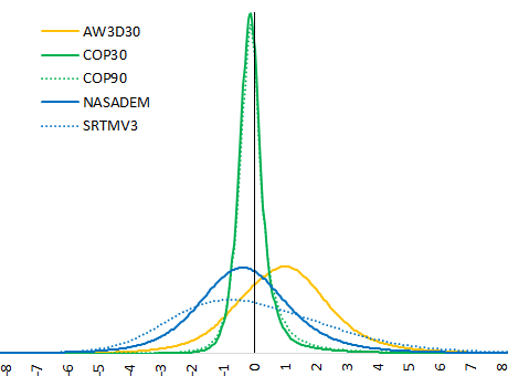
| DEM | Comparisons | RMSE | Mean | StDev | < 2 m | > 8 m |
|---|---|---|---|---|---|---|
| ASTER | 45,115,623 | 9.44 | -3.91 | 8.59 | 20.6% | 32.1% |
| AW3D30 | 45,115,596 | 2.68 | 1.09 | 2.45 | 69.6% | 0.9% |
| COP30 | 45,115,640 | 1.20 | 0.12 | 1.20 | 97.0% | 0.4% |
| COP90 | 45,115,640 | 1.26 | 0.15 | 1.25 | 95.8% | 0.3% |
| NASADEM | 29,583,548 | 2.38 | -0.23 | 2.37 | 75.9% | 1.2% |
| SRTMV3 | 28,703,799 | 2.82 | 0.15 | 2.81 | 57.3% | 1.2% |
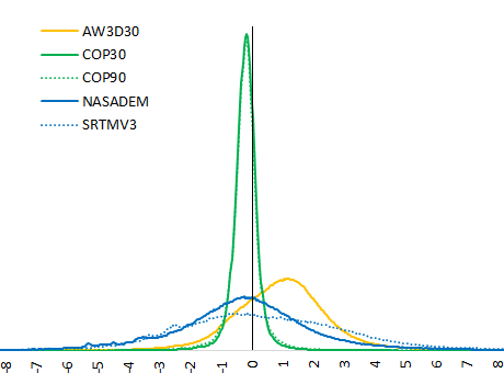
| DEM | Comparisons | RMSE | Mean | StDev | < 2 m | > 8 m |
|---|---|---|---|---|---|---|
| ASTER | 6,111,147 | 12.13 | -6.92 | 9.96 | 13.3% | 49.5% |
| AW3D30 | 6,111,143 | 3.34 | 1.07 | 3.16 | 72.1% | 1.3% |
| COP30 | 6,111,149 | 1.22 | -0.12 | 1.21 | 98.5% | 0.3% |
| COP90 | 6,111,149 | 1.30 | -0.12 | 1.29 | 97.6% | 0.3% |
| NASADEM | 1,183,242 | 4.72 | -0.08 | 4.72 | 65.5% | 3.3% |
| SRTMV3 | 1,144,267 | 4.30 | 0.55 | 4.27 | 52.9% | 3.1% |
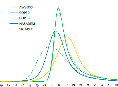
| DEM | Comparisons | RMSE | Mean | StDev | < 2 m | > 8 m |
|---|---|---|---|---|---|---|
| ASTER | 13,035,290 | 9.05 | -3.44 | 8.38 | 17.7% | 35.4% |
| AW3D30 | 13,035,290 | 3.61 | 1.84 | 3.10 | 59.2% | 3.8% |
| COP30 | 13,035,290 | 3.26 | 1.50 | 2.90 | 74.3% | 3.9% |
| COP90 | 13,035,290 | 3.23 | 1.56 | 2.82 | 72.2% | 3.6% |
| NASADEM | 9,574,430 | 3.16 | 0.13 | 3.16 | 73.3% | 3.1% |
| SRTMV3 | 8,724,611 | 3.14 | 0.06 | 3.14 | 59.1% | 2.5% |
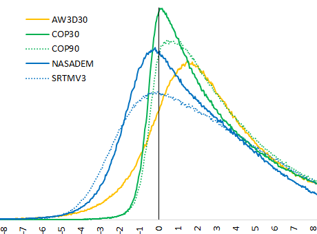
| DEM | Comparisons | RMSE | Mean | StDev | < 2 m | > 8 m |
|---|---|---|---|---|---|---|
| ASTER | 3,181,084 | 9.04 | 0.80 | 9.00 | 18.4% | 34.6% |
| AW3D30 | 3,181,084 | 6.18 | 3.87 | 4.82 | 35.4% | 15.9% |
| COP30 | 3,181,084 | 6.12 | 3.99 | 4.64 | 42.9% | 16.2% |
| COP90 | 3,181,084 | 5.99 | 4.08 | 4.38 | 38.3% | 15.5% |
| NASADEM | 2,871,974 | 4.25 | 2.00 | 3.75 | 49.1% | 6.7% |
| SRTMV3 | 2,826,930 | 5.06 | 2.64 | 4.32 | 40.6% | 11.0% |
| DEM | Comparisons | RMSE | Mean | StDev | < 2 m | > 8 m |
|---|---|---|---|---|---|---|
| ASTER | 2,170,635 | 9.24 | -0.01 | 9.24 | 18.3% | 35.2% |
| AW3D30 | 2,170,635 | 5.95 | 3.83 | 4.56 | 37.1% | 15.2% |
| COP30 | 2,170,635 | 6.16 | 4.02 | 4.67 | 42.9% | 17.1% |
| COP90 | 2,170,635 | 6.05 | 4.12 | 4.44 | 38.9% | 16.7% |
| NASADEM | 1,726,060 | 4.00 | 1.71 | 3.62 | 53.2% | 5.3% |
| SRTMV3 | 1,682,947 | 4.37 | 1.99 | 3.89 | 47.9% | 7.3% |
| DEM | Comparisons | RMSE | Mean | StDev | < 2 m | > 8 m |
|---|---|---|---|---|---|---|
| ASTER | 1,890,159 | 8.24 | -0.79 | 8.20 | 23.9% | 24.2% |
| AW3D30 | 1,890,159 | 3.61 | 1.91 | 3.07 | 50.2% | 2.6% |
| COP30 | 1,890,159 | 2.86 | 1.26 | 2.57 | 76.4% | 2.5% |
| COP90 | 1,890,159 | 2.86 | 1.38 | 2.50 | 73.3% | 2.3% |
| NASADEM | 1,877,695 | 3.14 | 0.68 | 3.07 | 62.6% | 2.1% |
| SRTMV3 | 1,875,576 | 4.07 | 1.66 | 3.72 | 45.1% | 4.7% |
All DEMs show significant positive elevation bias in broadleaf and mixed forests, measuring well above the forest floor. However, we use DEMs for wireless propagation studies, where hills and trees block wireless signals. So we welcome this positive bias, as long as it does not extend above the forest canopy. For you, this bias might be a concern — it all depends on your use case.
Geoid DEM elevations were converted to WGS84 ellipsoid elevations before being compared to ICESat-2 elevations. Gridded data (ie. DEM and vertical datum conversion) used 16-value bicubic interpolation. SRTM / NASADEM had fewer comparisons because their coverage does not extend north of 60N and 61N latitude, respectively.
Please contact us if you you have any questions about our study.